Genre

I first count the number of movies on various subjects, and comedies and action movies are the most.

movies_count <- movies %>%  # assigning a variable 
  group_by(genre) %>% # grouping the movie dataset by genre
  summarize(movies_count = n()) %>%  # using the summarise function to count the no of movies in each genre
  slice_max(order_by = movies_count, n = 10) %>%
  ggplot(aes(x = movies_count, 
             y = fct_reorder(genre, movies_count))) +
  geom_col() +
  theme_bw() +
  labs(title = "Movies by Genre")

movies_count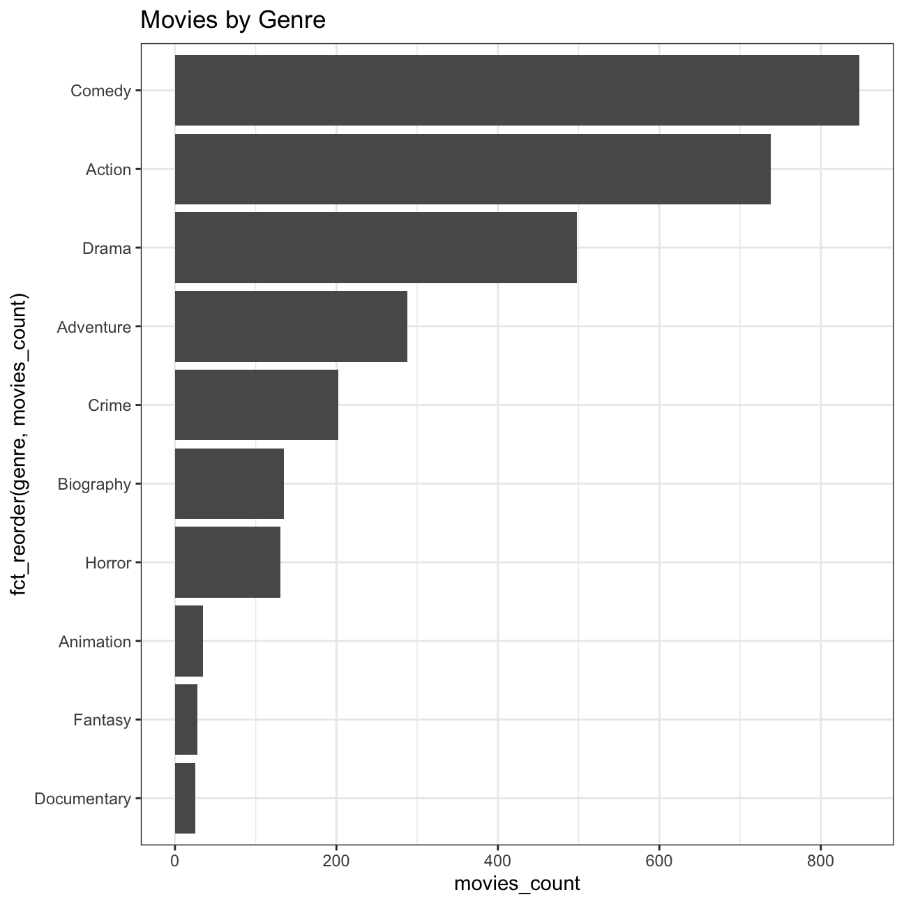

Then I also want to look at the gross and budget of these movies.

• Produce a table with the average gross earning and budget (gross and budget) by genre. Calculate a variable return_on_budget which shows how many $ did a movie make at the box office for each $ of its budget. Ranked genres by this return_on_budget in descending order.

avg_gross_earning_plot <- movies %>%
  group_by(genre) %>% 
  summarize(avg_gross_earning = mean(gross),
            avg_budget = mean(budget),
            return_on_budget = avg_gross_earning/avg_budget) %>%
  slice_max(order_by = return_on_budget, n = 10) %>%
  ggplot(aes(x = return_on_budget, 
             y = fct_reorder(genre, return_on_budget))) +
  geom_col() +
  theme_bw() +
  labs(title = "Returns by Genre",
       x = "Return on budget",
       y = "Genre")

avg_gross_earning_plot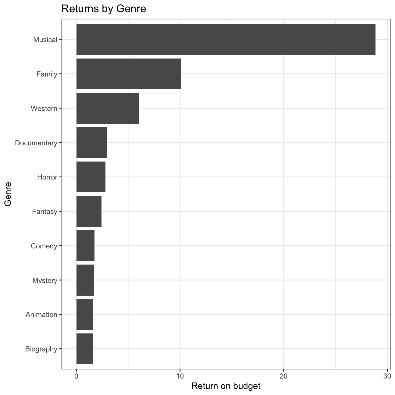

In terms of return on budget, we can see that musical genre has the highest return. That is partly because low budget is needed for such kind of movies - you don’t need many expensive props (eg. cars, skyscrapers), and not too much money to spend in post production to get fancy special effects.

Directors

Let’s take a look about what the top 15 directors who have created the highest gross revenue in the box office.

movies %>%  
    group_by(director) %>%  
    summarize(total_gross_amount = sum(gross),
        mean_gross_amount = mean(gross),
        median_gross_amount = median(gross), 
        standard_deviation_gross_amount = sd(gross)) %>%
    slice_max(order_by = total_gross_amount, n=15) 

## # A tibble: 15 × 5
##    director          total_gross_amount mean_gross_amount median_gross…¹ stand…²
##    <chr>                          <dbl>             <dbl>          <dbl>   <dbl>
##  1 Steven Spielberg          4014061704        174524422.     164435221   1.01e8
##  2 Michael Bay               2231242537        171634041.     138396624   1.27e8
##  3 Tim Burton                2071275480        129454718.      76519172   1.09e8
##  4 Sam Raimi                 2014600898        201460090.     234903076   1.62e8
##  5 James Cameron             1909725910        318287652.     175562880.  3.09e8
##  6 Christopher Nolan         1813227576        226653447      196667606.  1.87e8
##  7 George Lucas              1741418480        348283696      380262555   1.46e8
##  8 Robert Zemeckis           1619309108        124562239.     100853835   9.13e7
##  9 Clint Eastwood            1378321100         72543216.      46700000   7.55e7
## 10 Francis Lawrence          1358501971        271700394.     281666058   1.35e8
## 11 Ron Howard                1335988092        111332341      101587923   8.19e7
## 12 Gore Verbinski            1329600995        189942999.     123207194   1.54e8
## 13 Andrew Adamson            1137446920        284361730      279680930.  1.21e8
## 14 Shawn Levy                1129750988        102704635.      85463309   6.55e7
## 15 Ridley Scott              1128857598         80632686.      47775715   6.88e7
## # … with abbreviated variable names ¹​median_gross_amount,
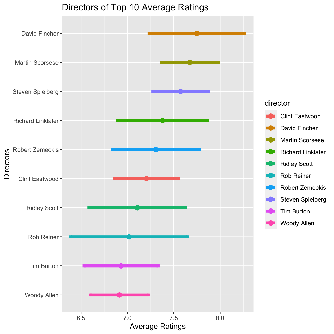
## #   ²​standard_deviation_gross_amount

Are the differences in ratings in line with differences in gross? Let’s have a look.

ci_interval <- movies %>%
  group_by(director) %>% 
  summarize(avg = mean(rating),
            sd =sd(rating),
            count = n(),
            se = sd / sqrt(count),
            t_critical = qt(0.975, count-1),
            lower = avg - se *t_critical,
            upper = avg + se *t_critical) %>% 
  filter(count >= 10) %>%
  slice_max(order_by = avg, n = 10) %>%
  ggplot(aes(x = avg, y = fct_reorder(director, avg))) +
  geom_point(aes(x = avg, color = director), size = 3) +
  geom_errorbar(aes(xmin = lower, xmax = upper, color = director), width = 0.1, size = 2) +
  labs(title = "Directors of Top 10 Average Ratings",
       x = "Average Ratings",
       y = "Directors")

ci_interval